The Shadow

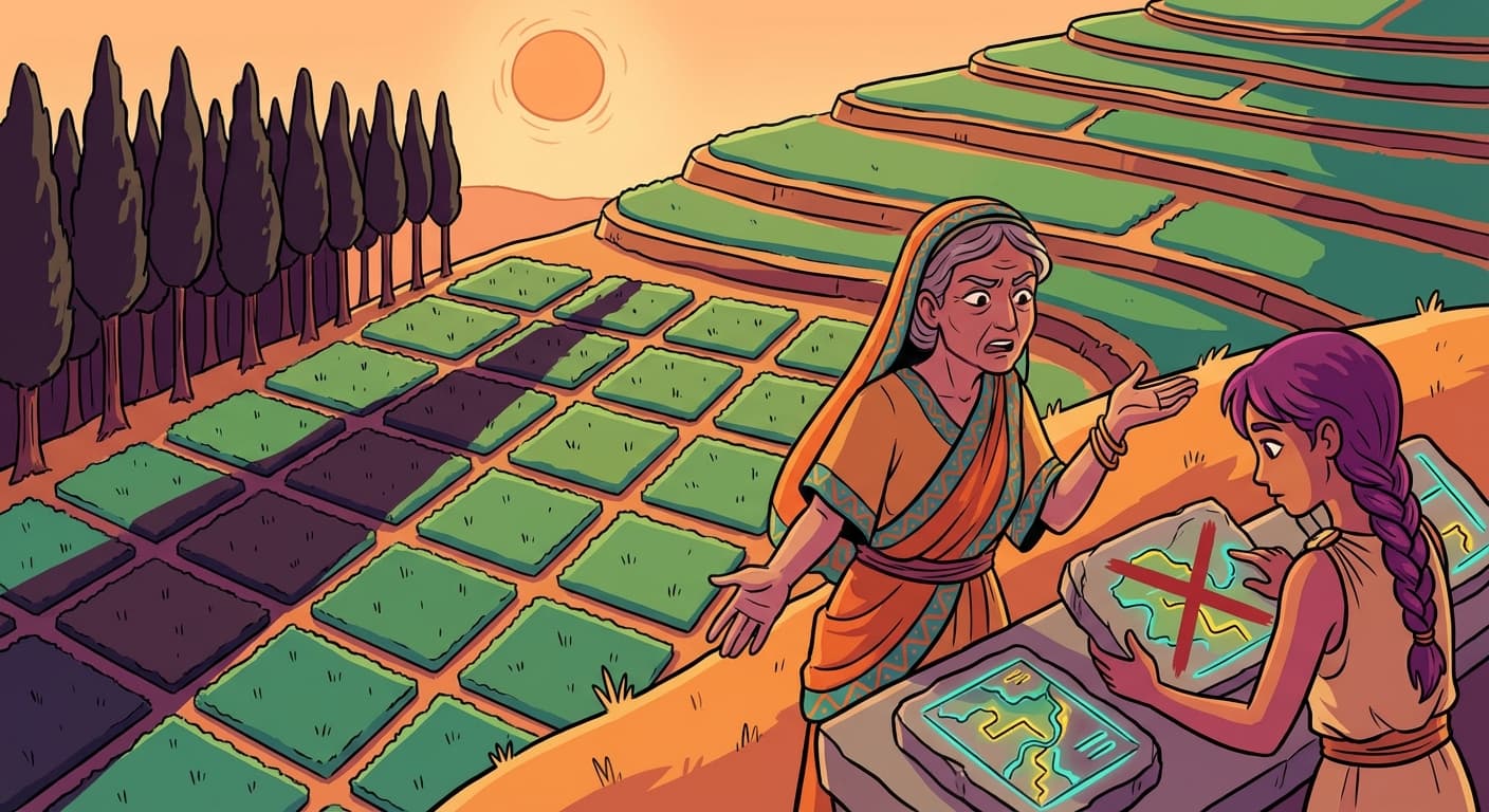
The convolutional pipeline worked well for Kvrothja's standard fields. But she had a more ambitious request.

Kvrothja: Some fields have complex blight patterns — not just simple clusters but long streaks along irrigation channels, or ring-shaped patterns where the blight started at a central source and radiated outward. The simple filters detect patches, but they miss these larger structures.

A 3×3 filter could detect a local cluster — a small patch of blight. But a streak that stretched across ten plots, or a ring with a radius of five plots, was far larger than the filter's window. The filter could see the individual segments of the streak but could not recognise the streak as a coherent pattern.

Stacking Layers

Trviksha's solution was to stack convolutional layers. The first layer's filters scanned the raw field and detected simple, local features — edges, spots, transitions between healthy and blighted plots. The feature maps from the first layer were then fed into a second layer of filters.

The second layer's filters did not scan the raw field. They scanned the first layer's feature maps — the processed output. A 3×3 filter in the second layer looked at a 3×3 patch of the first layer's output. But each cell of the first layer's output already summarised a 3×3 patch of the raw input. So the second layer's effective view covered roughly a 5×5 region of the original field.

After pooling, the second layer's view expanded further. And a third layer, stacked on top, could see an even wider region — combining the first layer's local features into the second layer's intermediate features into the third layer's high-level structures.

Trviksha: The first layer sees edges. The second layer sees shapes made of edges — curves, corners, lines. The third layer sees structures made of shapes — streaks, rings, clusters with specific profiles. Each layer combines the previous layer's features into more complex patterns.

Blortz: Like reading. The first layer sees strokes. The second layer sees letters made of strokes. The third layer sees words made of letters. Each layer builds on the one below it.

The Deep Network

Trviksha built a three-layer convolutional network:

Layer 1: Eight 3×3 filters, producing eight feature maps. Pooling. Layer 2: Sixteen 3×3 filters (scanning the pooled feature maps from Layer 1), producing sixteen feature maps. Pooling. Layer 3: Thirty-two 3×3 filters, producing thirty-two feature maps. Pooling.

The output of the third layer — thirty-two heavily compressed feature maps — fed into a standard hidden layer that produced the final classification.

The network was deep: three convolutional layers, each building features from the previous layer's features. Total weights: roughly two thousand — far fewer than the six thousand of the fully connected approach, but distributed across a hierarchy of increasingly abstract features.

On the training fields, the deep network achieved 93% accuracy. On held-out test fields, 91%. The deep architecture was capturing the complex spatial patterns that the single-layer convolutional network had missed.

Kvrothja: It detects the streaks along the channels. It detects the ring patterns. It even detects a pattern I had not consciously noticed — blight tends to form along the downhill edge of terraces where water collects.

The Healthy Field

Then Field 34 came through.

Field 34 was perfectly healthy. No blight whatsoever. Kvrothja had surveyed it personally. Every plot was green and productive.

The network classified it as high-risk. The prediction was confident — the network was nearly as certain that Field 34 was diseased as it was about fields with actual blight.

Kvrothja: Field 34 is one of my healthiest fields. There is no blight. Your model is wrong.

Trviksha: The model is very confident. Something in the field is triggering the blight detectors.

She examined the network's intermediate feature maps for Field 34 — what each layer was "seeing." The first layer had detected a set of strong edges running diagonally across the field. The second layer had combined these edges into a streak pattern. The third layer had classified the streak as a blight channel — the same pattern it had learned from fields where blight followed irrigation channels.

But Field 34 had no blight. The edges were not blight boundaries. They were shadows — cast by a row of tall trees along the western edge of the field during the afternoon survey. The shadow created a visual pattern on the survey grid (the surveyor had recorded "shadow-obscured" plots as ambiguous, which the encoding treated similarly to "partially blighted"). The first layer could not tell the difference between "dark because blighted" and "dark because shadowed." It had detected a genuine pattern in the input data — dark edges — and passed it along. The deeper layers had elaborated this into a confident but completely wrong diagnosis.

A field grid where a diagonal shadow from a row of trees creates a dark streak across healthy plots. The network's feature maps show the streak being detected as an edge (Layer 1), combined into a channel pattern (Layer 2), and classified as blight (Layer 3). Kvrothja gestures at the healthy field in frustration while Trviksha examines the feature maps

The Lesson

Trviksha: The network learned to detect blight from patterns in the data. But the patterns it found are not always blight. A shadow creates the same local pattern as a disease boundary. The network cannot tell the difference because both look the same at the level of a 3×3 patch.

Blortz: The network sees what it was trained to see. It was trained on fields where dark edges meant blight. It learned "dark edges mean blight." It did not learn "dark edges caused by disease mean blight, but dark edges caused by shadows do not." It does not know what shadows are.

Kvrothja: Can you fix it?

Trviksha: I can include shadowed fields in the training data, labelled as healthy. Then the network will learn that some dark-edge patterns are not blight. But there will always be features in the data that the network treats as meaningful but that have nothing to do with the actual phenomenon. The model sees patterns. It does not understand what causes them.

This was the deeper lesson of the feature hierarchy. Each layer of the deep network built increasingly complex and abstract features — edges, shapes, structures. But "complex" and "abstract" did not mean "correct." The features were statistical regularities in the training data, not facts about the world. A pattern that correlated with blight in the training fields — dark edges — was not necessarily caused by blight. The network had no access to causation. It had only correlation, layered and refined through successive layers, but correlation nonetheless.

Glagalbagal: The pebbles do not know what they are counting.

Trviksha: They never did. But the more layers we add, the easier it is to forget that.

Trviksha has built a deep convolutional neural network — multiple convolutional layers stacked so that each layer detects increasingly complex features. The first layer finds simple local patterns (edges, spots). The second layer combines these into intermediate structures (shapes, curves). The third layer combines those into complex, high-level features (streaks, rings, structures). This feature hierarchy is how modern image recognition systems work — the same architecture that powers face detection, medical imaging, and self-driving car vision. But the shadow incident illustrates a fundamental limitation: the network learns features that are statistically associated with the target, not features that causally determine it. If shadows and blight both create dark edges, the network cannot distinguish them without seeing examples of both. This problem — models relying on spurious correlations — remains one of the most active research areas in machine learning. Think about a time you made a wrong assumption because two things usually went together: if it is dark outside, it is usually night — but during an eclipse, that assumption fails. The network's "eclipse" was a shadow.